Pytorch入门
[TOC]
环境配置
|
|
查看cuda版本:
|
|
根据cuda版本进行选择:Pytorch本地安装
|
|
安装检测
|
|
此时说明安装成功
前言
法宝函数
|
|
Dataset
以蜜蜂蚂蚁数据集进行说明
其文件目录:
|
|
子文件夹小附有若干张jpg
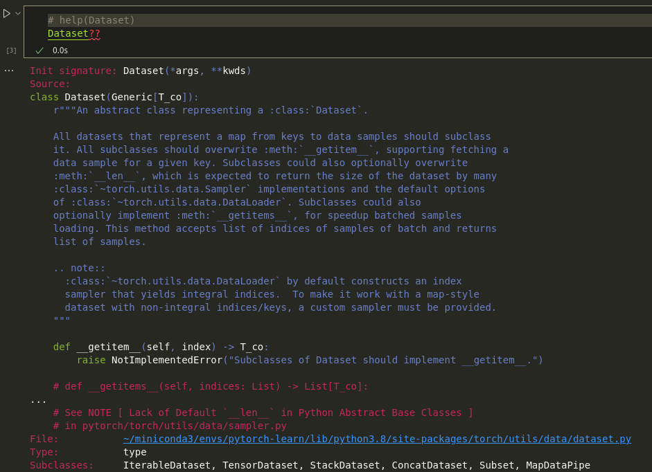
接下来我们需要使用torch的Dataset去加载数据集
| An abstract class representing a :class:
Dataset. |
| All datasets that represent a map from keys to data samples should subclass | it. All subclasses should overwrite :meth:__getitem__, supporting fetching a | data sample for a given key. Subclasses could also optionally overwrite | :meth:__len__, which is expected to return the size of the dataset by many | :class:~torch.utils.data.Samplerimplementations and the default options | of :class:~torch.utils.data.DataLoader. Subclasses could also | optionally implement :meth:__getitems__, for speedup batched samples | loading. This method accepts list of indices of samples of batch and returns | list of samples.
省流:
- 需要继承
- 必须重写
__getitem__ - 可以重写
__len__
|
|
写法非常自由,你只要保证重写的函数返回正确结果即可
Tensorboard
|
|
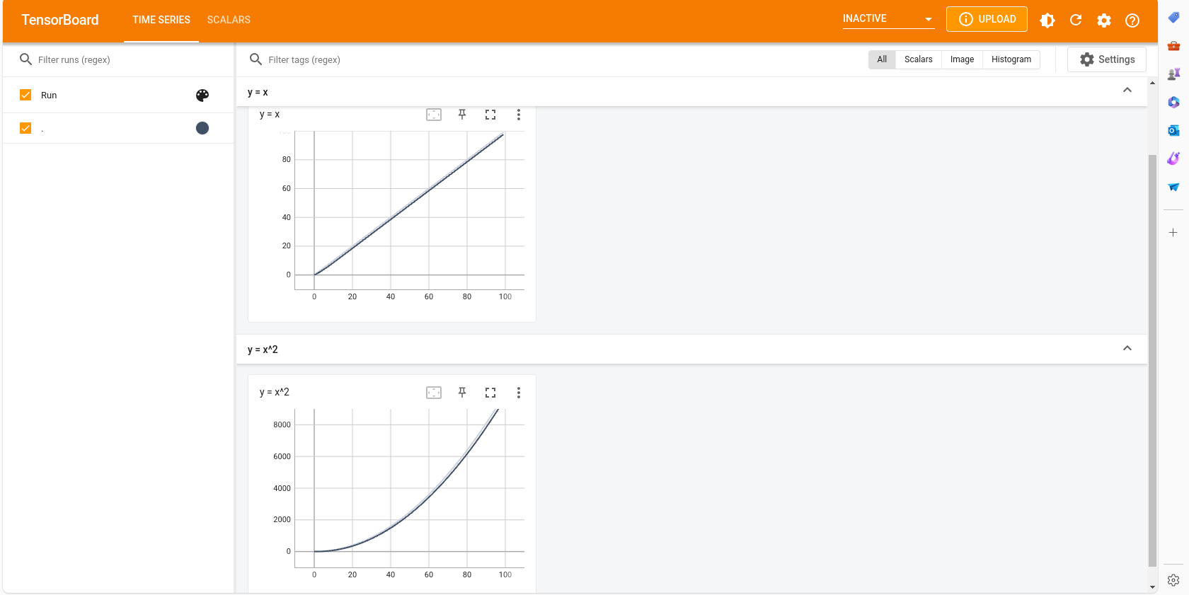
Scalars
绘制一些图表,观察训练的loss变化
|
|
在终端中:
|
|
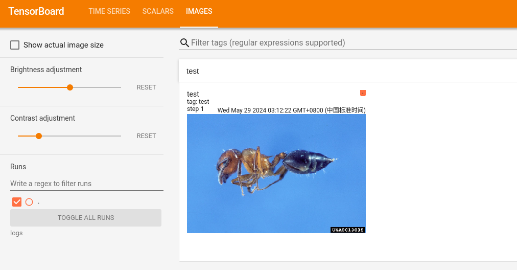
Images
可视化实际的训练效果,上传图片进行展示
|
|
Transforms
留个印象就好,能通过这个方法对数据、图片等进行互相转换、变化
常见的有:
- ToTensor:转化为Tensor数据
- Normalize:归一化
- Resize:对图片数据进行缩放
- Compose:用列表记录多个变化,进行一次性操作
可能用到的时候查一下就行
适合对多个数据同时进行相同的处理
Torchvision数据集的下载与使用
|
|
此时我们得到的数据集都是(PIL对象,标签索引)
我们可以使用Transform统一把图片转化为Tensor,方便Pytorch使用
最简单的方法:
|
|
DataLoader
|
|
网络
|
|
卷积层
对于一张H*W的RGB图片,其通道数channel为3
我们使用多少个卷积核,就会产生多少个out_channels
|
|
池化层
卷积后的图像依旧比较大,可以通过池化层进行压缩
避免过拟合、去除冗余
|
|
我们可以喂入图片,就可以得到压缩画质版本的输出
激活层
|
|
其他
- 正则化层
- 线性层……
Sequential
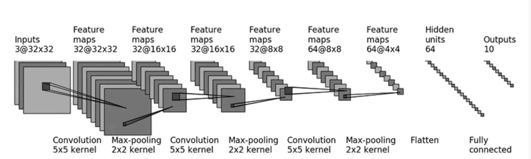
我们试图构建一个较大的网络对CIFAR10数据集进行推理
|
|
损失函数
|
|
反向传播
|
|
优化器
|
|
我们可以进行多轮学习
|
|
当loss收敛后,就完成了训练
模型的修改
除了自己的模型,其实也能修改别人训练完的模型
以此网络为例:
|
|
网络结构为:
|
|
添加
|
|
修改
|
|
模型的保存与读取
save
|
|
完整保存了模型的结构与参数,数据量大
state_dict(官方推荐)
|
|
GPU训练
- 损失函数
- 数据
- 模型
三种对象直接x = x.cuda()即可放入GPU显存
但是若GPU不存在,此时代码兼容性一般
|
|
更推荐这种写法
完整流程
|
|
构建网络
|
|
初始化
|
|
训练
|
|